Speech Synthesis with suno-ai/bark
When you think of speech synthesis, you might think of a very robotic-sounding voice, like this one from 1979. Maybe you think of more modern voice assistants, like Siri or the Google Assistant. While these are certainly improvements over what we had in the 1970s, they still wouldn’t be mistaken for recordings of actual humans. Enter Bark text-to-speech, a generative AI model like Stable Diffusion or ChatGPT developed by Suno AI. Like these other generative models, Bark takes a text prompt and creates something new. However, it doesn’t produce images or more text. From their GitHub page: “Bark can generate highly realistic, multilingual speech as well as other audio – including music, background noise and simple sound effects. The model can also produce nonverbal communications like laughing, sighing and crying.”
This is a fundamental departure from previous generations of speech synthesis. Bark does not try to break down text into phonemes for recreation by a recorded voice. Rather, it “predicts” what an audio recording might be like, based on the text it’s given. The result is much more natural sounding speech and other conversational sounds. Bark is also an important generative AI model because it is freely available for commercial use, and can run on very modest hardware, including consumer GPUs with minimal vRAM.
We set out to benchmark Bark across a range of consumer hardware configurations using Salad’s GPU Cloud.
Benchmarking Bark text-to-speech model on Consumer GPUs
You know we like to keep things food-related here at Salad, so we selected this Food.com Recipe Dataset from Kaggle, a collection of a couple hundred thousand recipes, along with reviews of those recipes. We’re going to have Bark read these recipes out for us. If you’d like to follow along, we’ll be working with Python 3.10 throughout this project.
Unlike some of our other benchmarks, our goal here is not to demonstrate that SaladCloud is the most cost-effective platform for AI inference. Rather, we want to leverage some unique capabilities of Salad’s distributed cloud to evaluate Bark’s performance across a wide range of consumer GPUs. And, if I’m being totally honest, I just thought this would be a fun project.
You can skip straight to the outputs if that’s what you’re here for.
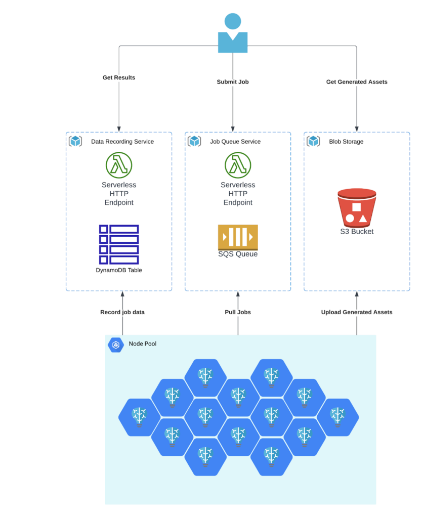
Architecture
We’ll be using our standard batch processing framework for this, the same we’ve used for many other benchmarks, including Whisper Large and SDXL.
Data Preparation
First, we need to download our dataset. Kaggle is free, but does require an account. Once you have an account, you’ll need to grab your API token from your account settings.

Clicking the “Create New Token” button will initiate a download of a file called kaggle.json. Place the file in your home directory at ~/.kaggle/kaggle.json. This will allow you to authenticate requests with the Kaggle CLI.
pip install kaggle
kaggle datasets download -d shuyangli94/food-com-recipes-and-user-interactions
unzip "food-com-recipes-and-user-interactions.zip" -d "food-com-recipes-and-user-interactions"
Now we have a folder called food-com-recipes-and-user-interactions that contains the following files:
.
├── ingr_map.pkl
├── interactions_test.csv
├── interactions_train.csv
├── interactions_validation.csv
├── PP_recipes.csv
├── PP_users.csv
├── RAW_interactions.csv
└── RAW_recipes.csv

0 directories, 8 files
Our first step is to load up our recipes and interactions in a pandas DataFrame. This step may take several minutes.
import pandas as pd
recipes = pd.read_csv('food-com-recipes-and-user-interactions/RAW_recipes.csv')
reviews = pd.read_csv('food-com-recipes-and-user-interactions/RAW_interactions.csv')
Let’s take a peek and see what we’re working with.
recipes.head(5)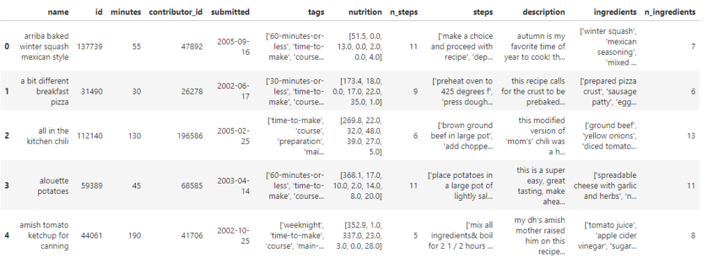
recipes.info()<class 'pandas.core.frame.DataFrame'>
RangeIndex: 231637 entries, 0 to 231636
Data columns (total 12 columns):
# Column Non-Null Count Dtype
--- ------ -------------- -----
0 name 231636 non-null object
1 id 231637 non-null int64
2 minutes 231637 non-null int64
3 contributor_id 231637 non-null int64
4 submitted 231637 non-null object
5 tags 231637 non-null object
6 nutrition 231637 non-null object
7 n_steps 231637 non-null int64
8 steps 231637 non-null object
9 description 226658 non-null object
10 ingredients 231637 non-null object
11 n_ingredients 231637 non-null int64
dtypes: int64(5), object(7)
memory usage: 21.2+ MBOk, so we have 231,637 recipes, with fields like “id”, “name”, “description”, and “steps”. There’s some other fields as well, but we won’t be using them for this project. Let’s check out our review data.
reviews.head(5)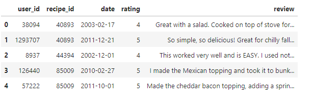
reviews.info()<class 'pandas.core.frame.DataFrame'>
RangeIndex: 1132367 entries, 0 to 1132366
Data columns (total 5 columns):
# Column Non-Null Count Dtype
--- ------ -------------- -----
0 user_id 1132367 non-null int64
1 recipe_id 1132367 non-null int64
2 date 1132367 non-null object
3 rating 1132367 non-null int64
4 review 1132198 non-null object
dtypes: int64(3), object(2)
memory usage: 43.2+ MBIn our review data, we have 1,132,367 reviews, each of which has a “recipe_id” and a “rating.” Let’s see our top recipes by average review:
top_recipes = reviews.groupby('recipe_id').agg(average_rating=('rating', 'mean')).sort_values(by='average_rating', ascending=False).reset_index()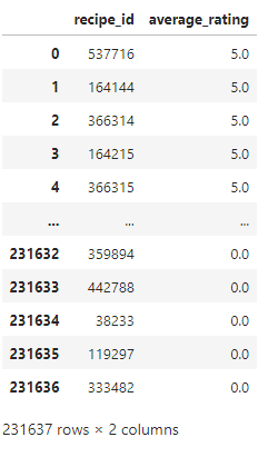
Interestingly, we see a lot of recipes with an average rating of 0.0. Maybe we should filter this down to only recipes with “good” reviews, over 4.5.
filtered_recipes = top_recipes[top_recipes['average_rating'] >= 4.5]
Ok, now we’ve got 144,177 recipes that have received an average rating of at least 4.5. Now we can merge this table into the recipe table, and get a collection of recipe data, but only for recipes with a rating of at least 4.5.
merged_recipes = pd.merge(filtered_recipes, recipes, left_on='recipe_id', right_on='id', how='inner')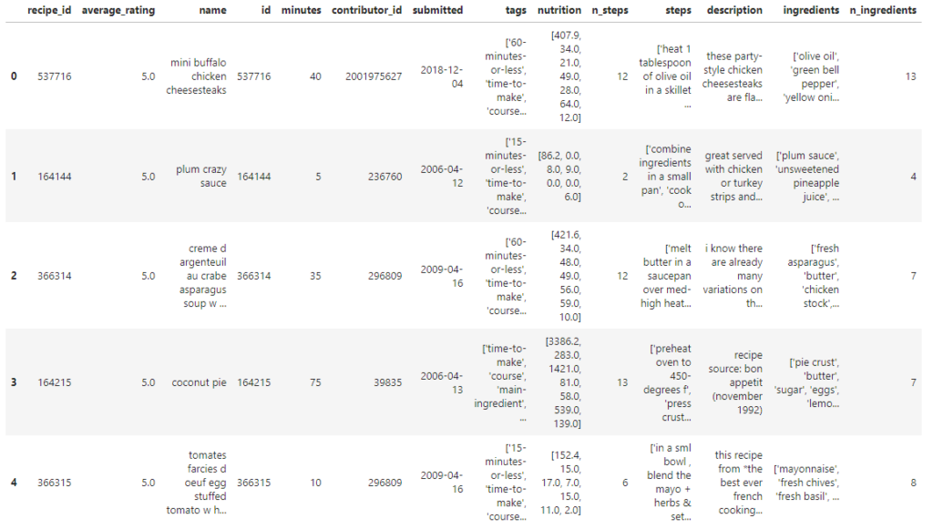
One thing to note here is that although steps look like a list of strings, it is, in fact, just a string.
merged_recipes["steps"][0]"['heat 1 tablespoon of olive oil in a skillet over medium heat', 'add bell pepper and saut until softened slightly , about 3 minutes', 'add onion and season with salt and pepper', 'saut until softened , about 7 minutes', 'stir in the chicken', 'add heavy cream , buffalo sauce and blue cheese', 'stir and cook until heated through , about 3-5 minutes', 'season with salt and pepper', 'turn heat to low and keep warm', 'microwave the cheez whiz in a heat safe bowl for about 90 seconds , stirring every 30 seconds', 'wrap the rolls in damp paper towels and microwave for 90 seconds', 'fill each roll with buffalo chicken mixture , drizzle with warm cheeze whiz , and garnish with green onions , parsley and blue cheese crumbles']"Since our goal is to write a “script” for Bark to read, we’re going to want these strings parsed into lists. We’re going to use the ast module to safely evaluate these strings into python lists.
import ast
merged_recipes["steps"] = merged_recipes['steps'].apply(ast.literal_eval)
merged_recipes["steps"][0]['heat 1 tablespoon of olive oil in a skillet over medium heat',
'add bell pepper and saut until softened slightly , about 3 minutes',
'add onion and season with salt and pepper',
'saut until softened , about 7 minutes',
'stir in the chicken',
'add heavy cream , buffalo sauce and blue cheese',
'stir and cook until heated through , about 3-5 minutes',
'season with salt and pepper',
'turn heat to low and keep warm',
'microwave the cheez whiz in a heat safe bowl for about 90 seconds , stirring every 30 seconds',
'wrap the rolls in damp paper towels and microwave for 90 seconds',
'fill each roll with buffalo chicken mixture , drizzle with warm cheeze whiz , and garnish with green onions , parsley and blue cheese crumbles']Ok, now we need to turn this data into a “script”: something that will sound a little more natural when Bark reads it. I admit that I was tempted to use a large language model (LLM) like Llama 2 for this, and the results would have likely been better and sound more natural. However, for the sake of expediency, I’m just going to use a simple python function to stitch each row into a script.
def recipe_script(row):
    # Start by introducing the recipe by name
    intro = f"Today, we're going to make {row['name']}."

    # Mention the cooking time
    time_to_cook = f"This dish will take approximately {row['minutes']} minutes to prepare and cook."

    # Share the description if it exists
    description = f"{row['description']}" if not pd.isna(row['description']) else ""

    # Define some transitions for the steps
    transitions = [
        "Next, ",
        "After that, ",
        "Following that, ",
        "Then, ",
        "Subsequently, ",
        "Once done, ",
        "Now, "
    ]

    steps = row["steps"]

    # Convert the list of steps into a string with transitions
    steps_with_transitions = []
    for i, step in enumerate(steps):
        # Add a transition if it's not the last step
        if i < len(steps) - 1:
            transition = transitions[i % len(transitions)]  # Cycle through transitions
            steps_with_transitions.append(step + ". " + transition)
        else:
            # No transition for the last step
            steps_with_transitions.append(step + ".")

    steps_script = " ".join(steps_with_transitions)

    # Combine all parts to make the full script
    full_script = f"{intro} {time_to_cook} {description} {steps_script}"

    return full_script
Let’s test it on our first row.
sample_row = merged_recipes.iloc[0]  # Taking the first row as an example
script = recipe_script(sample_row)
print(script)"Today, we're going to make mini buffalo chicken cheesesteaks. This dish will take approximately 40 minutes to prepare and cook. these party-style chicken cheesesteaks are flavored with buffalo sauce and blue cheese and garnished with fresh herbs. a heavy drizzle of cheez whiz really takes it to a new level. heat 1 tablespoon of olive oil in a skillet over medium heat. Next, add bell pepper and saut until softened slightly , about 3 minutes. After that, add onion and season with salt and pepper. Following that, saut until softened , about 7 minutes. Then, stir in the chicken. Subsequently, add heavy cream , buffalo sauce and blue cheese. Once done, stir and cook until heated through , about 3-5 minutes. Now, season with salt and pepper. Next, turn heat to low and keep warm. After that, microwave the cheez whiz in a heat safe bowl for about 90 seconds , stirring every 30 seconds. Following that, wrap the rolls in damp paper towels and microwave for 90 seconds. Then, fill each roll with buffalo chicken mixture , drizzle with warm cheeze whiz , and garnish with green onions , parsley and blue cheese crumbles."This will be good enough for this project. We can see there are some typos in the original data, and it’ll be interesting to see how Bark handles those. However, we have a new problem now, which is that Bark works best with about 13 seconds of spoken text. Our script is quite a bit longer than that, so we’re going to have to chop it up into smaller chunks.
According to a quick Google search, the average speaking rate is 2.5 words per second, which would translate to a maximum of 32.5 words that Bark will happily do in one clip. Let’s round that down to 30, just to be safe. However, we don’t just want to split the script every 30 words. Ideally, we would only include whole sentences for each segment so that Bark can do a better job of tone and cadence. There are Natural Language Processing (NLP) techniques to do this with greater accuracy, but again, for expediency, we’re going to do this the simple way.
import re

def split_script(script, max_words=30):
    # Split the script into sentences
    sentences = re.split(r'(?<=[.!?])\s+', script)

  sections = []
  current_section = []
  current_word_count = 0

  for sentence in sentences:
      sentence_word_count = len(sentence.split())

      if current_word_count + sentence_word_count <= max_words:
          current_section.append(sentence)
          current_word_count += sentence_word_count
      else:
          # Add the current section to sections if it's not empty
            	      if current_section:
                	sections.append(" ".join(current_section).strip())

            	      # Start a new section with the current sentence
                    current_section = [sentence]
                    current_word_count = sentence_word_count

    # Add any remaining sentences to sections
    if current_section:
        sections.append(" ".join(current_section).strip())

    return sections
Let’s see how that works:
sections = split_script(script, max_words=30)
for section in sections:
    print(section)
    print("-" * 50)
Today, we're going to make mini buffalo chicken cheesesteaks. This dish will take approximately 40 minutes to prepare and cook.
--------------------------------------------------
these party-style chicken cheesesteaks are flavored with buffalo sauce and blue cheese and garnished with fresh herbs. a heavy drizzle of cheez whiz really takes it to a new level.
--------------------------------------------------
heat 1 tablespoon of olive oil in a skillet over medium heat. Next,  add bell pepper and saut until softened slightly , about 3 minutes.
--------------------------------------------------
After that,  add onion and season with salt and pepper. Following that,  saut until softened , about 7 minutes. Then,  stir in the chicken.
--------------------------------------------------
Subsequently,  add heavy cream , buffalo sauce and blue cheese. Once done,  stir and cook until heated through , about 3-5 minutes. Now,  season with salt and pepper.
--------------------------------------------------
Next,  turn heat to low and keep warm. After that,  microwave the cheez whiz in a heat safe bowl for about 90 seconds , stirring every 30 seconds.
--------------------------------------------------
Following that,  wrap the rolls in damp paper towels and microwave for 90 seconds.
--------------------------------------------------
Then,  fill each roll with buffalo chicken mixture , drizzle with warm cheeze whiz , and garnish with green onions , parsley and blue cheese crumbles.
--------------------------------------------------
Ok, that’s pretty good. Let’s move forward with this solution. Bark includes a large number of voice presets, but since our data is all English, we’re going to use just the English language voices. There’s 10 of those, numbered 0-9. We’ll use a simple function to randomly select a voice for each recipe.
import random

def get_random_voice():
    speaker_id = random.randint(0, 9)  # Select a random number between 0 and 9 inclusive
    return f"v2/en_speaker_{speaker_id}"
The final thing we need is to create signed upload URLs for the audio clips that will be generated by Bark. A signed url is a URL that includes a time-limited authentication token allowing a client to upload a specific file. This is often preferable to giving clients long-lived credentials.
We’ll be using AWS S3 to store all of our generated audio files. At this point, we don’t really know how long a given URL will need to stay active, so we’re going to set the maximum expiration time of 7 days (604,800 seconds). If you are using temporary credentials, such as those in a Sagemaker notebook, the expiration will only be good for as long as your current credentials are good. Make sure you generate your URLs using credentials that expire after you want the URL to expire.
import boto3

s3 = boto3.client('s3')

def generate_presigned_upload_url(bucket_name, object_name, expiration=604800):
    """
    Generate a pre-signed URL to upload a file to S3.

    :param bucket_name: Name of the S3 bucket.
    :param object_name: Name of the S3 object (typically filename).
    :param expiration: Time in seconds for the pre-signed URL to remain valid.
    :return: Pre-signed URL as string, or None if error.
    """
    try:
        response = s3.generate_presigned_url(
            'put_object',
            Params={'Bucket': bucket_name, 'Key': object_name},
            ExpiresIn=expiration
        )
    except Exception as e:
        print(e)
        raise e

    return response
Using all these pieces, we can now make a generator function that transforms our DataFrame into generation jobs for Bark, and load those jobs into AWS SQS, which we’ll be using for our work queue.
sqs = boto3.client('sqs')

# Use your own bucket and queue info here
bucket = "salad-benchmark-public-assets"
prefix = "recipe-audio/"
queue_url = "https://sqs.us-east-2.amazonaws.com/000000000000/benchmark-recipes-to-read.fifo"

def generate_jobs(df):
    for _, row in df.iterrows():
        script = recipe_script(row)
        script_sections = split_script(script)
        voice = get_random_voice()
        for index, section in enumerate(script_sections):
            job = {
                "id": row["id"],
                "voice": voice,
                "script_section": section,
                "section_index": index,
                "upload_url": generate_presigned_upload_url(bucket, f"{prefix}{row['id']}/{index}.mp3")
            }
            yield job

def send_batch(sqs_queue_url, batch):
    entries = [
        {"Id": str(uuid.uuid4()), "MessageBody": json.dumps(job), "MessageGroupId": str(uuid.uuid4()), "MessageDeduplicationId": str(uuid.uuid4()) }
        for job in batch
    ]
    response = sqs.send_message_batch(QueueUrl=sqs_queue_url, Entries=entries)

    # Handle possible failed messages here (if needed)
    if 'Failed' in response:
        for failed in response['Failed']:
            print(f"Failed to send message {failed['Id']}: {failed['Message']}")


def send_jobs_to_sqs(sqs_queue_url, jobs_generator):
    # This will store the current batch of jobs
    batch = []
    for job in jobs_generator:
        batch.append(job)

        # If we have 10 jobs in the batch, send them
        if len(batch) == 10:
            send_batch(sqs_queue_url, batch)

            # Clear the batch for the next set of jobs
            batch.clear()

    # Send any remaining jobs in the batch (less than 10)
    if batch:
        send_batch(sqs_queue_url, batch)
Now we start loading our data. This will take a short while, as there are more than a million jobs to be generated from our 144k recipes.
send_jobs_to_sqs(queue_url, generate_jobs(merged_recipes))The jobs we generate look like this:
{'id': 537716,
  'voice': 'v2/en_speaker_0',
  'script_section': "Today, we're going to make mini buffalo chicken cheesesteaks. This dish will take approximately 40 minutes to prepare and cook.",
  'section_index': 0,
  'upload_url': 'https://salad-benchmark-public-assets.s3.amazonaws.com/recipe-audio/537716/0.mp3?X-Amz-Algorithm=AWS4-HMAC-SHA256&X-Amz-Credential=ASIAXTWUXWKJN7Z7OIOS%2F20230922%2Fus-east-2%2Fs3%2Faws4_request&X-Amz-Date=20230922T160126Z&X-Amz-Expires=604800&X-Amz-SignedHeaders=host&X-Amz-Security-Token=IQoJb3JpZ2luX2VjECAaCXVzLWVhc3QtMiJIMEYCIQDyhAo%2BwCEnomY%2F4q%2FeRtwVPP7vXt5mED3zd3CtA00KMgIhAJ6kamgfqtLYsYkDsCOaDaa8d1z5snlUwrpfHfacOWfMKrQCCBkQABoMNTIzMzU4NDE3NTU0IgwZVBAvZX65EBuy%2Fl0qkQKCC4XEjpvemQuLQYarRNRUfAvrNKb1xVhadjuH2yRxR%2BgeJveSjj7KUlyj8GePDT8MCQvfA3w2Zy1yVl3DX6YPsKtpBhADEV7gUUTAP8bHrF%2F1xuiwer6JYGulR4uSYmSfV6nWN2H2djm2QXvYW2qBi4bH0yYvc5Ll8XSD126zGqZr7%2FDJM2RvZv1Rm9pKp76a0tLOfiz%2BDfu%2F68Ybjln38vFPMk7RKmxfS5SIeoMHJ8vmjH6cbBN3Xg2R18tXeDbMPNYu1%2FX4cvNMNKLNMNpoKeEZh4nWN2EqTDaf%2BxYdm7q3KVlouneLZc8vcxsGT2L%2Be8zX9TL8SnqNSlkz%2BtoJD%2F%2BdIkc0wjuhIuQ9r6o%2BzPAwkvO2qAY6kgEabkNaA2U1N7ifg%2FxxXDX35HouLoIxVfigFk1XINWvw9LQlTNACFoeP2dQRDno4twgeBqF%2FzdjBQ7Q9kFVR6sUhNmwzlY%2BgHV2RmXoFKnV44kUxnPx7nIlS6EhZArnacojlUjKuzrGqnVz8b0yqOAhlEqA8VBov4iqS54gj74f9SzUYnkv5hKiH7LeJVg2%2FsaicQ%3D%3D&X-Amz-Signature=f1fbad2480bc2a350d90fb7696afb6ddfc2d4b83236f6714c310b39de11841c7'}
Text-to-Speech Inference Server
Next we need our inference server. I typically make these as minimalist as possible, and handle the queue logic in a different layer. You can see the code for our Bark inference server here. Although Bark does have it’s own python library, we’ll be using the Hugginface 🤗**Transformers** library, along with the 🤗Optimum library.
Setting up the model is very easy this way.
from transformers import AutoProcessor, AutoModel
from optimum.bettertransformer import BetterTransformer
import torch

def load(load_only=False):
    processor = AutoProcessor.from_pretrained("suno/bark")
    model = AutoModel.from_pretrained("suno/bark", torch_dtype=torch.float16)

    if not load_only:
        model.to("cuda")
        model = BetterTransformer.transform(model, keep_original_model=False)

    return processor, model
We offer the load_only argument in this function so that we can call it during the build process and not worry about moving it to the GPU or optimizing it at that time.
With our model loaded, we need a function to predict the audio from a given text input and voice.
import soundfile as sf
from pydub import AudioSegment
import numpy as np
from io import BytesIO


def predict(processor, model, text, voice_preset=None):
    # We need to convert our text into something the model can understand,
    # using the processor. We're going to have it return PyTorch tensors.
    inputs = processor(text, voice_preset=voice_preset, return_tensors="pt")

    # Now we need to move these tensors to the GPU, so they can be processed
    # by the model.
    inputs = {k: v.to("cuda") for k, v in inputs.items()}

    # The model generates more tensors that can be decoded into audio.
    speech_values = model.generate(**inputs, do_sample=True)

    # For interpreting the tensors back into audio, we need
    # to know the sampling_rate that was used to generate it.
    sampling_rate = model.generation_config.sample_rate

    # Now we need to move our tensors back to the CPU and convert them to a NumPy array
    speech = speech_values.cpu().numpy().squeeze()

    # The soundfile library requires us to convert our array of float16 numbers
    # into an array of int16 numbers.
    scaled_speech = np.int16(speech * 32767)

    # We don't want to actually write to the file system, so we'll create
    # a file-like BytesIO object, and write the wav to that
    wav = BytesIO()
    sf.write(wav, scaled_speech, sampling_rate, format="WAV", subtype="PCM_16")

    # WAV files are huge, so we're going to use pydub to convert it to a much
    # smaller mp3 "file"
    audio = AudioSegment.from_wav(wav)
    dur_ms = len(audio)

    mp3 = BytesIO()
    audio.export(mp3, format="mp3")

    return mp3, dur_ms
The rest of our server is a very standard FastAPI app that is served with Uvicorn. It has 2 endpoints, a health check, and a generate endpoint.
from fastapi import FastAPI, HTTPException, Body
from starlette.responses import StreamingResponse
from typing import Optional
from pydantic import BaseModel

app = FastAPI()


class GenerateRequest(BaseModel):
    # Add your input parameters here
    text: str
    voice_preset: Optional[str] = None


@app.get("/hc")
async def health_check():
    return "OK"


@app.post("/generate", response_class=StreamingResponse)
def generate(req: GenerateRequest = Body(...)):
    try:
        mp3, dur_ms = predict(processor, model, req.text, req.voice_preset)
    except Exception as e:
        raise HTTPException(status_code=500, detail=str(e))

    return StreamingResponse(mp3, media_type="audio/mpeg")
This establishes a server where you can post a JSON request body with some text and a voice_preset, and it will send you an mp3 once it has been created.
Once our server has been built and run with Docker, we can test it with a simple cURL command.
curl  -X POST \
  'http://localhost:8000/generate' \
  --header 'Content-Type: application/json' \
  --data-raw '{
  "text": "My name is Suno, and uh - I am an artificial intelligence that generates sound from text. Can you tell, or do I sound human?",
  "voice_preset": "v2/en_speaker_4"
}' -o outputs/sample.mp3
You can download the pre-built Docker image here.
Queue Worker
On top of our inference server, we’re going to add a queue worker. I’ve implemented this one in typescript. If you’ve read code from my other benchmarks, you’ll notice a striking similarity between this and my others. Essentially, we have a main loop that fetches work from a queue, submits that work to our Bark inference server, and asynchronously uploads the generated mp3, records the job in the job recording service, and marks the job complete. You can see the code in more detail here. Frankly, this is the least interesting part of this project, so we’re not going to dive into too much detail in this post.
The completed Docker image containing both the inference server and the queue worker can be found here.
Setting up the Container Group on SaladCloud
While you can certainly set this up using the Portal, I’m going to use the public API, since I will be creating multiple nearly identical groups. The “Create Container Group” endpoint is well documented.
I’m going to request 200 nodes, using 2 container groups of 100 nodes each (a platform limit). I’ll be making 2 post requests with a body like this:
{
  "name": "bark-1",
  "container": {
    "image": "saladtechnologies/bark-benchmark:latest",
    "resources": {
      "cpu": 2,
      "memory": 8192,
      "gpu_class": "Stable Diffusion Compatible"
    },
    "environment_variables": {
      "BENCHMARK_SIZE": "-1",
      "REPORTING_URL": "https://someurl.com",
      "QUEUE_URL": "https://someotherurl.com",
      "REPORTING_API_KEY": "An API key used with our reporting and queue services",
      "BENCHMARK_ID": "bark-recipes-1",
      "QUEUE_NAME": "recipes-to-read"
    }
  },
  "replicas": 100
}
Bark has very modest hardware requirements, so we’ve selected 2 CPUs and 8GB of RAM. For our GPU, we’ve selected SaladCloud’s “Stable Diffusion Compatible” GPU class, which is perfect for our goal of evaluating performance across a wide variety of GPUs. Using this setting will allow our containers to be allocated to any node with a GPU that has at least 8GB of vRAM.
It’s also kind of an incredible value, as it costs only $0.08/hr, no matter what GPU you actually get. Some of the nodes will end up with RTX 3060 GPUs, but others will end up with RTX 4090 GPUs and everything in between. If your workloads are not terribly latency-sensitive, this is a fantastic option for minimizing the per-inference cost and perfect for a large batch processing job like we’ve set up.
Analyzing and Compiling the Bark Benchmark Results
Almost exactly 2 days later, the task is completed, and we’ve got 1,065,674 audio clips to work with. We’ll be using pandas, plotly, and pydub to work with the results. We will also need ffmpeg and ffprobe installed to work with the mp3 files.
Let’s set up our dependencies.
pip install pydub ffmpeg
curl https://johnvansickle.com/ffmpeg/releases/ffmpeg-release-amd64-static.tar.xz -o ffmpeg.tar.xz \
     && tar -xf ffmpeg.tar.xz && rm ffmpeg.tar.xz
sudo cp ffmpeg-6.0-amd64-static/ffmpeg /usr/bin/ffmpeg
sudo cp ffmpeg-6.0-amd64-static/ffprobe /usr/bin/ffprobe
Our data is all in DynamoDB, so we’re going to create a simple generator function to paginate through our benchmark results and convert them into rows for our pandas dataframe.
import boto3
import json
import pandas as pd

dynamodb = boto3.client("dynamodb", region_name="us-east-2")

def query_dynamodb_table(benchmark_id):

    # Initial query parameters
    query_params = {
        'TableName': 'benchmark-data',  # replace with your table name
        'KeyConditionExpression': 'benchmark_id = :benchmarkValue',
        'IndexName': "benchmark_id-timestamp-index",
        'ExpressionAttributeValues': {
            ':benchmarkValue': {"S": benchmark_id}
        }
    }

    while True:
        # Execute the query
        response = dynamodb.query(**query_params)
        # Yield each item
        for item in response['Items']:
            yield item

        # If there's more data to be retrieved, update the ExclusiveStartKey
        if 'LastEvaluatedKey' in response:
            query_params['ExclusiveStartKey'] = response['LastEvaluatedKey']
        else:
            break

def get_rows_for_pd():
    for item in query_dynamodb_table("bark-recipes-1"):
        timestamp = item["timestamp"]["N"]
        data = json.loads(item["data"]["S"])
        system = data["system_info"]
        del data["system_info"]

        row = {
            **data,
            **system,
            "timestamp": timestamp
        }
        yield row

df = pd.DataFrame(get_rows_for_pd())
We’re going to go ahead and make a couple extra columns, one for word count, and one to convert our Epoch ms timestamp into a python datetime object. The timestamp column marks when the generation was completed, and logged in the database.
# 1. Counting the number of words in the 'script_section'
df['word_count'] = df['script_section'].str.split().str.len()

# Convert the timestamp to datetime
df['timestamp'] = pd.to_datetime(df['timestamp'].astype(int), unit='ms')
Now we have a DataFrame to work with:
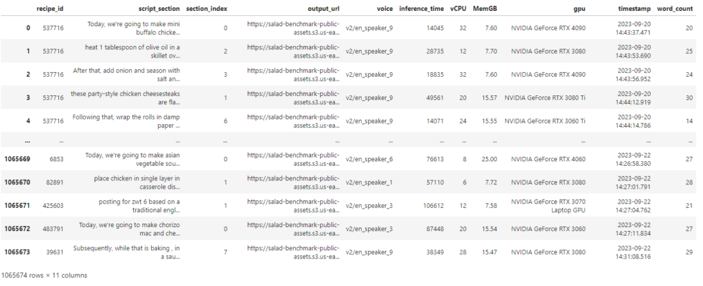
What is notably lacking from this dataset right now is the length of each generated clip, and of course, we’ll need to recombine all of the script sections back into a single audio file reading the entire script. With over a million clips (47GB) to download and analyze, memory efficiency will be important to consider, especially since the machine I’m doing the analysis on only has 16GB of RAM. We won’t be able to load all 1 million clips in memory at the same time, but we do want to get the length of each clip and add it as a column to our dataframe.
First, we’ll make a function that retrieves the mp3 file and returns it as a pydub.AudioSegment, along with the length of the clip in ms. Like before, we’re going to download these files into a BytesIO object rather than saving each clip to the file system.
from pydub import AudioSegment
import aiohttp
import asyncio
import nest_asyncio
from io import BytesIO

# If you're running a jupyter notebook, you need this
nest_asyncio.apply()

# We're going to limit ourselves to 50 simultaneous downloads
semaphore = asyncio.Semaphore(50)

async def fetch_clip_async(url):
    async with semaphore:
        async with aiohttp.ClientSession() as session:
            async with session.get(url) as response:
                response.raise_for_status()
                content = await response.read()
                clip = AudioSegment.from_file(BytesIO(content), format="mp3")
                return clip, len(clip)
We also want a function that will grab every clip for a given recipe, get the length of them, and stitch them together into a single file.
async def process_recipe_group_async(group):
    # Fetch all clips concurrently and get their lengths
    clips_and_lengths = await asyncio.gather(*[fetch_clip_async(url) for url in group['output_url'].tolist()])
    clips, clip_lengths = zip(*clips_and_lengths)  # unzip the results

    # Sort clips by section_index and concatenate
    sorted_clips = [clip for _, clip in sorted(zip(group['section_index'].tolist(), clips))]
    combined_clip = sum(sorted_clips, AudioSegment.empty())

    # Save the concatenated clip
    recipe_id = group['recipe_id'].iloc[0]
    combined_clip.export(f"audio/combined_audio_{recipe_id}.mp3", format="mp3")

    # Return a dictionary of {section_index: clip_length}
    return {section_index: clip_len for section_index, clip_len in zip(group['section_index'], clip_lengths)}tion_index'], clip_lengths)}
This function saves each completed clip in a directory called “audio” with a filename like “combined_audio_123456.mp3” for each unique recipe ID. We can use our DataFrame to group the clips together by recipe_id:
grouped = df.groupby('recipe_id')Now, we can start the long process of downloading and processing all of these clips. I considered building out another batch process to run on SaladCloud for this but decided it was out of scope for this project. Instead, we’ll just loop through the recipe groups and save our progress periodically in case this Sagemaker notebook has any problems (which it definitely will). This may look overly complicated for a download script, but there’s a surprising amount that can and will go wrong when you’re dealing with large numbers of files. If you assume 99.99% of downloads succeed, you will still have 100 failures for every million downloads.
def save_checkpoint(clip_lengths_dict, processed_count):
    """Save the current state of clip_lengths_dict to a file."""
    filename = f"clip_length_checkpoint.json"
    checkpoint_path = os.path.join("recipe-checkpoints", filename)
    with open(checkpoint_path, 'w') as f:
        json.dump(clip_lengths_dict, f)
        print(f"Checkpoint saved with {processed_count} recipes evaluated.")


async def process_with_retry_async(group, max_retries=3, base_delay=1):
    retries = 0
    while retries <= max_retries:
        try:
            return await process_recipe_group_async(group)
        except Exception as e:
            if retries == max_retries:
                raise e
            retries += 1
            await asyncio.sleep(base_delay * (2 ** retries))


async def process_group_parallel_async(group):
    recipe_id = str(group['recipe_id'].iloc[0])
    if recipe_id in clip_lengths_dict:
        return None

    try:
        result = await process_with_retry_async(group)
        return (recipe_id, result)
    except Exception as e:
        print(f"Error processing recipe_id {recipe_id} after retries: {e}")
        return None


clip_lengths_dict = {}  # Dict to store {recipe_id: {section_index: clip_length}}
async def process_all_recipes():
		global clip_lengths_dict
    processed_count = len(clip_lengths_dict.keys())

    # Create tasks directly from the grouped DataFrameGroupBy object
    tasks = [process_group_parallel_async(group_data) for _, group_data in grouped if str(group_data['recipe_id'].iloc[0]) not in clip_lengths_dict]

    # Use as_completed to process tasks as they complete
    for completed_task in asyncio.as_completed(tasks):
        try:
            result = await completed_task
            if result is not None:
                recipe_id, group_result = result
                clip_lengths_dict[recipe_id] = group_result
                processed_count += 1

                # Save a checkpoint every 5k recipes
                if processed_count % 5000 == 0:
                    save_checkpoint(clip_lengths_dict, processed_count)

        except Exception as e:
            # This catch block is for unexpected errors outside of process_group_parallel_async
            print(f"Unexpected error: {e}")

    save_checkpoint(clip_lengths_dict, processed_count)

loop = asyncio.get_event_loop()
loop.run_until_complete(process_all_recipes())
loop.close()
While this runs for the next several hours, we are recombining all of our clips into whole recipes and populating our dictionary clip_lengths_dict with the length of each clip. Now, it’s time to turn that data into an extra column on our dataframe.
df['clip_length'] = df.apply(lambda row: clip_lengths_dict[row['recipe_id']][row['section_index']], axis=1)Now, with this data, we can calculate some interesting metrics, such as “How many seconds of speech can we generate per second of inference?”. A value of 1.0 would indicate a real-time processing speed, where 1 second of audio is created with 1 second of compute. Higher numbers indicate better performance. We’ll also add a couple more columns, such as “words spoken per second of compute.”
# Seconds of Speech generated per second
df["speed_s_generated_per_s"] = df["clip_length"] / df["inference_time"]

# 2. Convert 'inference_time_seconds' from milliseconds to seconds
df['inference_time_seconds'] = df['inference_time'] / 1000.0

# 3. Calculate words per second
df['words_per_second'] = df['word_count'] / df['inference_time_seconds']
Let’s find out how many GPU types we managed to collect data on.
unique_gpus = df['gpu'].unique().tolist()
unique_gpus
['NVIDIA GeForce RTX 4090',
'NVIDIA GeForce RTX 3080',
'NVIDIA GeForce RTX 3080 Ti',
'NVIDIA GeForce RTX 3060 Ti',
'NVIDIA GeForce RTX 4070',
'NVIDIA GeForce RTX 3090',
'NVIDIA GeForce RTX 4060 Laptop GPU',
'NVIDIA GeForce RTX 3070',
'NVIDIA GeForce RTX 3060',
'NVIDIA GeForce RTX 4070 Ti',
'NVIDIA GeForce RTX 3070 Laptop GPU',
'NVIDIA GeForce RTX 4060 Ti',
'NVIDIA GeForce RTX 4080',
'NVIDIA GeForce RTX 4070 Laptop GPU',
'NVIDIA GeForce RTX 3080 Ti\nNVIDIA GeForce RTX 3060 Ti',
'NVIDIA GeForce RTX 4060',
'NVIDIA GeForce RTX 3080 Laptop GPU',
'NVIDIA GeForce RTX 3070 Ti Laptop GPU',
'NVIDIA GeForce RTX 3070 Ti',
'NVIDIA GeForce RTX 3080 Ti Laptop GPU',
'NVIDIA GeForce RTX 4090 Laptop GPU',
'NVIDIA GeForce RTX 3060 Ti\nNVIDIA GeForce RTX 3060 Ti',
'NVIDIA GeForce RTX 4080 Laptop GPU',
'NVIDIA GeForce RTX 3090 Ti',
'NVIDIA GeForce RTX 3060\nNVIDIA GeForce RTX 2080 Ti',
'NVIDIA GeForce RTX 3060\nNVIDIA GeForce GTX 1070',
'NVIDIA GeForce GTX 1050 Ti\nNVIDIA GeForce RTX 3060',
'NVIDIA GeForce RTX 3080 Ti\nNVIDIA GeForce GTX 1060 6GB',
'NVIDIA GeForce RTX 3060\nNVIDIA GeForce GTX 1060 3GB',
'NVIDIA GeForce RTX 3060\nNVIDIA GeForce RTX 3060',
'NVIDIA GeForce GTX 745\nNVIDIA GeForce RTX 3060',
'NVIDIA GeForce GTX 970\nNVIDIA GeForce RTX 3070']For most of the visualizations we’re about to do, I want the results sorted by GPU class, from least powerful to most powerful. We’re going to make a couple imperfect assumptions to do this:
- Higher-numbered cards are more powerful. i.e., RTX 3080 is more powerful than RTX 3060.
- Cards with “Ti” in the name are more powerful than their non-ti counterparts. i.e. RTX 3080 Ti is more powerful than RTX 3080.
- Laptop versions of cards are less powerful than their desktop counterparts. i.e. RTX 3080 Ti Laptop is less powerful than RTX 3080 Ti.
We can use these rules to make a function that assigns a performance score to each GPU:
import re

def performance_score(gpu_name):
    # Extract the number part using regex
    match = re.search(r'(\d+)', gpu_name)
    if match:
        number = int(match.group(1))
    else:
        return 0  # Default performance score in case no number is found

    # Check for 'Ti', 'Laptop', and combinations
    if 'Ti' in gpu_name and 'Laptop' in gpu_name:
        return number + 0.3
    elif 'Ti' in gpu_name:
        return number + 0.5
    elif 'Laptop' in gpu_name:
        return number
    else:
        return number + 0.1
And we can use that to add a performance column to our dataframe.
# Creating a new column 'performance' based on the GPU's name
df['performance'] = df['gpu'].apply(performance_score)

# Sorting the dataframe based on the performance score
df_sorted = df.sort_values('performance')

df_sorted["gpu"] = df_sorted["gpu"].astype("category")
We’re going to use plotly to show us the distribution of inference speed for each gpu type, but first we’re going to pre-calculate that distribution with Pandas. Plotly can be excrutiatingly slow to render from large-ish dataframes.
# Group by 'gpu' and compute the statistics
grouped = df_sorted.groupby('gpu')['speed_s_generated_per_s']

q1 = grouped.quantile(0.25)
median = grouped.median()
q3 = grouped.quantile(0.75)

# Optionally, compute outliers (values below Q1 - 1.5*IQR or above Q3 + 1.5*IQR)
iqr = q3 - q1
# Function to detect outliers for each group
# Compute the lower and upper bounds for outliers
lower_bound = q1 - 1.5 * iqr
upper_bound = q3 + 1.5 * iqr

# Adjust the min and max values to exclude outliers
min_vals = grouped.apply(lambda group: group[group >= lower_bound[group.name]].min())
max_vals = grouped.apply(lambda group: group[group <= upper_bound[group.name]].max())

outliers = grouped.apply(detect_outliers).reset_index()

# Combine the computed statistics into a new dataframe
stats_df = pd.DataFrame({
    'min': min_vals,
    'q1': q1,
    'median': median,
    'q3': q3,
    'max': max_vals
}).reset_index()

stats_df.head(5)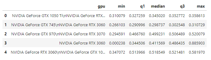
Now, we have a much smaller dataframe with the statistical summaries we want, and we can draw a box plot for it.
# Create a box plot using the precomputed statistics
traces = []
for index, row in stats_df.iterrows():
    trace = go.Box(
        y=[row['min'], row['q1'], row['median'], row['q3'], row['max']],
        name=shortened_names[row['gpu']],
        # boxpoints='all',  # show all points
        # jitter=0.3,  # spread out the data points for better visibility
        # pointpos=-1.8  # position of the data points relative to the box
    )
    traces.append(trace)

# Create the layout and show the plot
layout = go.Layout(title="Generation Speed by GPU",
                   xaxis_title="GPU",
                   yaxis_title="Speed (Seconds of Audio per Second of Inference)",
                   height=800,
                   width=1080)

fig = go.Figure(data=traces, layout=layout)
fig.show()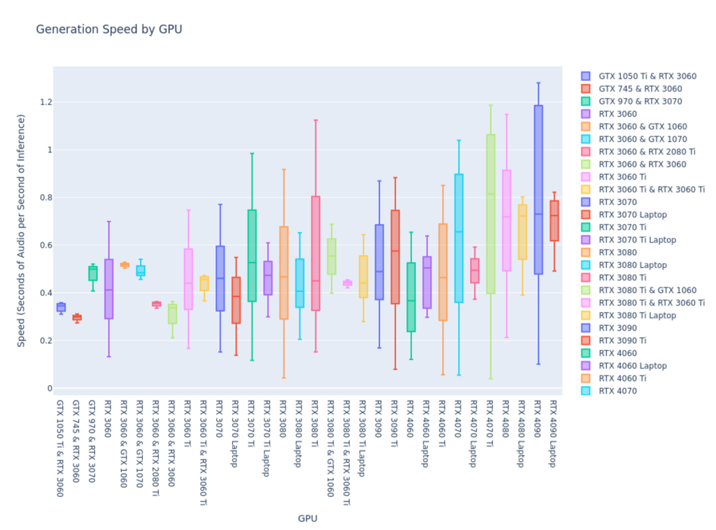
Right away, we can make a few observations:
- There is a significant range of performance, even across any one GPU type.
- Only a small set of GPUs ever reach a speed of 1.0, which is “real-time,” meaning 1 second of audio per second of inference: RTX 3080 Ti, RTX 4070, RTX 4070 Ti, RTX 4080, and RTX 4090.
- Laptop GPUs have considerably worse peak performance than their desktop counterparts but relatively similar medians and minimums.
This has me curious if the performance is similar for words per second rather than just the length of audio generated.
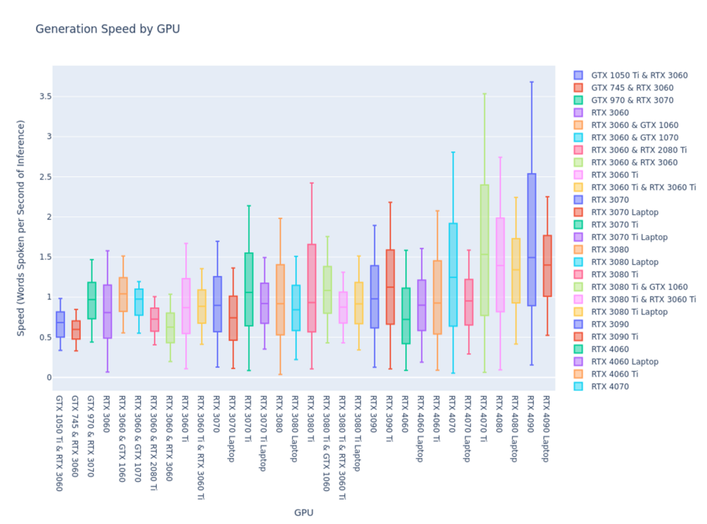
Yes, this box chart is remarkably similar in shape to the other, so I’d say we have a fairly accurate look at what kind of performance we can expect for any given GPU type.
Another thing I’m curious about is if a wider range of performance indicates a large sample size in the dataset. In other words, the range between minimum and maximum speed for the RTX 4090 is due to a disproportionate number of inferences performed by that GPU type.
# Group by GPU and count the number of inferences
gpu_counts = df_sorted['gpu'].value_counts().reset_index()
gpu_counts.columns = ['gpu', 'count']

gpu_counts['gpu'] = gpu_counts['gpu'].astype('category')
gpu_counts = gpu_counts.sort_values(by='gpu')

# Optionally, adjust the GPU names for better readability
gpu_counts['gpu'] = gpu_counts['gpu'].apply(lambda x: shortened_names[x] if x in shortened_names else x)

# Create a bar plot
fig = px.bar(gpu_counts, x='gpu', y='count', title="Number of Inferences by GPU",
             labels={'gpu': 'GPU', 'count': 'Number of Inferences'},
						 color_discrete_sequence=['#006400'])

fig.update_layout(height=800, width=1080)
fig.show()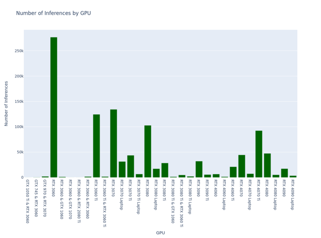
Well, we can reject that hypothesis, and in fact, I’m now curious if the opposite is true. Let’s graph the relationship between sample size and range size.
# Merge the two dataframes on the 'gpu' column
stats_df["gpu"] = stats_df['gpu'].apply(lambda x: shortened_names[x] if x in shortened_names else x)
merged_df = pd.merge(gpu_counts, stats_df, on='gpu')

# Compute the range for each GPU
merged_df['range'] = merged_df['max'] - merged_df['min']

fig = px.scatter(merged_df, x='count', y='range', title="Relationship between Sample Size and Data Distribution")
fig.update_layout(width=1080, height=800)
fig.show()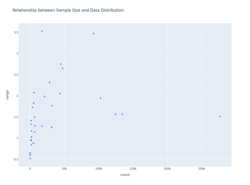
Looks like a very weak correlation. Let’s confirm.
correlation = merged_df['count'].corr(merged_df['range'])
print(f"The Pearson correlation coefficient between count and range is: {correlation:.2f}")
The Pearson correlation coefficient between count and range is: 0.27Ok, so we see a weak positive correlation between number of inferences and range of performance. From this we can assume that over time, we would see a slightly smaller range in performance for any given GPU, but should still expect a pretty large range.
Now that we’ve got a relatively good idea of inference speed across different GPUs, the remaining question is which one provides the best cost performance. We’ll be using SaladCloud’s pricing to evaluate this.
# The base cost for 2 CPUs and 8GB Ram
base_cost = 0.016
# A dictionary with the cost of each gpu type
gpu_cost = { ... }

# A new column for the hourly cost
stats_df['cost_per_hour'] = stats_df['gpu'].map(gpu_cost) + base_cost

# Compute cost per word for each interval
intervals = ['min', 'q1', 'median', 'q3', 'max']
seconds_per_hour = 3600
for interval in intervals:
    words_per_hour = stats_df[interval] * seconds_per_hour
    stats_df[f'words_per_dollar_{interval}'] = words_per_hour / stats_df['cost_per_hour']

# Create boxplot using plotly
fig = go.Figure()

for gpu in stats_df['gpu'].unique():
    gpu_data = stats_df[stats_df['gpu'] == gpu]
    fig.add_trace(go.Box(
        y=[gpu_data[f'words_per_dollar_{interval}'].values[0] for interval in intervals],
        name=gpu,
    ))

fig.update_layout(title='Boxplot of Cost per Word for Each GPU',
                  yaxis_title='Words Per Dollar',
                  xaxis_title='GPU',
                  height=800,
                  width=1080)
fig.show()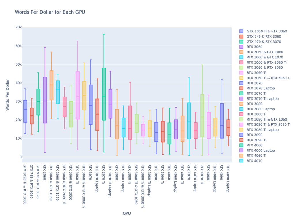
For a lot of use cases, this is going to be the most interesting chart here. Now we can see that although the latest cards are indeed much faster than older cards at performing the inference, there’s really a sweet spot for cost-performance in the lower end 30xx series cards.
Unanswered Questions
While we’ve learned a lot about the inference performance characteristics of the Bark model, what we don’t know is how good of a job it’s doing. It would be interesting to run a large transcription job on all of the generated audio, and determine how accurate Bark is at actually following the script.
In lieu of that, we’ve made available audio from 1000 top-rated recipes paired with the script it was trying to read.
Conclusions
- As is often the case, there’s a clear trade-off here between cost and performance. Higher-end cards are faster, but their disproportionate cost makes them more expensive per word spoken.
- The model’s median speed is surprisingly similar across GPU types, even though the peak performance can be quite different.
- SaladCloud has a lot of RTX 3060 GPUs available, based on their relatively low speed, yet a huge number of inferences were performed over the test.
- No matter what GPU you select, you should be prepared for significant variability in performance.
- Qualitative: While Bark’s speech is often impressively natural sounding, it does have a tendency to go off script sometimes.
Future Improvements
- Replace S3 with R2, an S3-compatible object storage service from Cloudflare that is less expensive and has no egress fees. This is ideal for a distributed cloud like SaladCloud, where all of the nodes are “outside” of Cloudflare or AWS.
- Modify the Bark server to return the length of the generated clip in a header. This way, we could record the length of each clip as it’s being generated, and we wouldn’t have to download all of the clips to get this information. We would still have to download all the clips to stitch them back together, but that could be done as a separate process.
- Implement a batch job to run on SaladCloud to join all the clips together. Downloading short clips and stitching them together into longer clips could have been done much faster in a highly parallel fashion.
- Use an open language model like Llama 2 to write better scripts from each recipe.
Salad suggests: If you are just looking to generate AI voices, give Veed.io’s AI voice generator a try. With AI voices and AI avatars, Veed.io will generate ultra-realistic text-to-speech audio/video for personal and commercial use.